介绍了 Pandas 中的 Index,Series, Dataframe 及其基本操作。
概念介绍
Index
Index 对象主要保存了关于轴的信息,index 对象类似数组,可以被切片,可以根据下标访问,但是不可以被修改;
可以通过 pd.Index 构造 index 对象,index 对象可以拥有重复的值。
index 比较常用的方法:
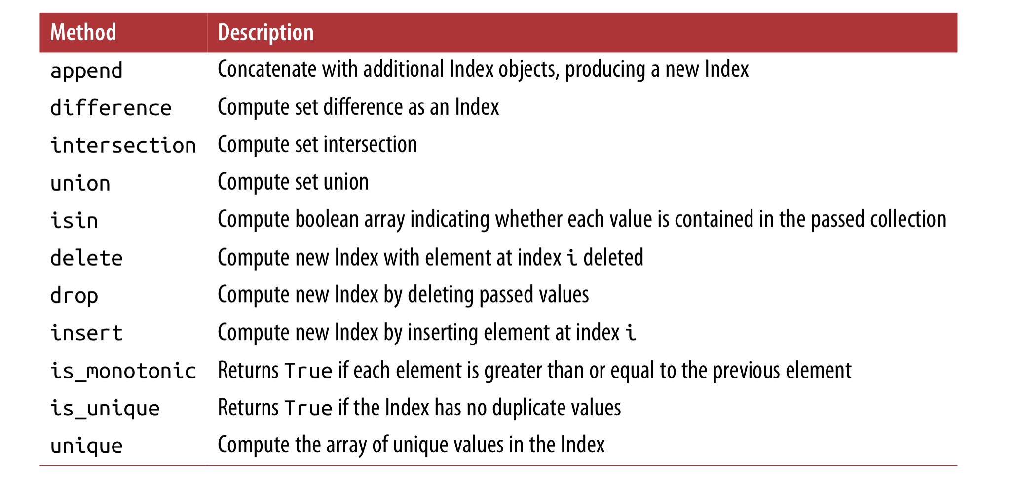
Series
Series 可以直接从数组初始化,如果没有指定 index,则会默认分配数字作为 index,也可以指定 index,但要求其长度与 values 一致。
当指定了 index 后,可直接通过 index 的名字访问 value,比如 obj['a'] 或者 obj[['a','b','c']],可以通过 obj[obj > 0] 的方式 filter其元素,或者进行运算:'a' in obj, obj * 2;
可以通过 dict 初始化 Series,结果的顺序与和 dict 中的 key 排序后的一样,如果像自定义顺序,可以在初始化函数中单独指定 index,需要保证传入的 index 在 dict 中的 key 中存在,否则会将值设为空。
多个 Series 在参与计算的时候,会自动对齐 index,有点类似 database 中的 join。
Series 对象本身和它的index 都有一个叫 name 的属性, index 可以被其它的值替代。
DataFrame
可以理解为 dict 中 value 为 Series,构造 dataframe 的方式也可以直接通过 dict,DataFrame 的 index 也和 Series 一样,会自动指定,column 的顺序也会重新排序,你也可以指定指定列的顺序,就像 Series 一样: pd.DataFrame(data, columns=[...]),如果你传的 columns 数组中,有 data 中没有的值,则会将该列添加到 DataFrame 中,值全部置空。
DataFrame 中的列,可以通过 df['a'] 或者 df.a 两种方式访问,将会返回一个 Series,第一种方式在任何情况下都可以使用,第二种方式则需要 column name 满足 python 对于变量名字的要求。从 DataFrame 拿到的 Series,将会拥有和 DataFrame 一样的 index,它的 name 属性也已经被自动设定。
DaFrame 中的行,也可以通过位置和名字访问,例如 loc 方法(之后介绍)。
给 Column 赋的值,可以是一个值,也可以是一个数组,或者 Series 对象。如果是数组,数组长度要与 dataframe 一致;如果是 Series,将按照 index label 赋值给 DataFrame; 给不存在的 column 赋值,会创建一个新的 column (只可以通过 ['column'] 的方式创建);
删除列,通过 del df['col'] 操作,但这种写法不鼓励,可以通过 df.drop(columns=['B', 'C'])。
DataFrame 的 column 和 index 都可以有 name, df.index.name = 'idx', df.columns.name = 'col', df.values 会返回一个 DataFrame 的值的二维数组。
Essential Functionality
Reindexing
reindex 是 pandas 里实现数据对齐的基本方法, 沿着指定轴,让现有数据匹配一组新标签,并重新排序。
可以在无数据但有标签的位置插入缺失值。
编写注重性能的代码时,最好花些时间深入理解 reindex:预对齐数据后,操作会更快。两个未对齐的 DataFrame 相加,后台操作会执行 reindex。
提取一个对象,并用另一个具有相同标签的对象 reindex 该对象的轴。这种操作的语法虽然简单,但未免有些啰嗦。这时,最好用 reindex_like() 方法,这是一种既有效,又简单的方式。
align() 方法是对齐两个对象最快的方式,该方法支持 join 参数,比如你想要根据 df2的列的顺序排序 df1 的列顺序 df1.align(df2, join='left'), axis=1。
可以直接调用 Series s.rename(str.upper) 来操作 index 上的 string 格式; 也可以操作 df 的 index 和 columns, df.rename({'one': 'foo', 'two': 'bar'}, axis='columns')。
reindex,ffill 与 bfill,在 reindex 时候产生的值用前、后的值去取代
1 | In [219]: rng = pd.date_range('1/3/2000', periods=8) |
上面的做法亦可通过 ts2.reindex(ts.index).fillna(method='ffill') 实现, 如果索引不是按递增或递减排序,reindex() 会触发 ValueError 错误。fillna() 与 interpolate() 则不检查索引的排序。limit 与 tolerance 参数可以控制 reindex 的填充操作。limit 限定了连续匹配的最大数量:
1 | In [229]: ts2.reindex(ts.index, method='ffill', limit=1) |
tolerance 限定了索引与索引器值之间的最大距离:
1 | In [230]: ts2.reindex(ts.index, method='ffill', tolerance='1 day') |
索引为 DatetimeIndex、TimedeltaIndex 或 PeriodIndex 时,tolerance 会尽可能将这些索引强制转换为 Timedelta,这里要求用户用恰当的字符串设定 tolerance 参数。
Dropping Entries from an Axis
如果有了 index,可以直接 index 名字删除某行 new_obj = obj.drop('c'), 或者同时删除多行 data.drop(['Colorado', 'Ohio']),axis=1 删除列,0 删除行。
代码示例
Indexing value
1 | # 使用中括号 |
Slicing DataFrames
1 | # eggs 列中的某些值 |
Filtering
1 | df.loc[:, df.all()] # 所有非0值 |
Understand Dataframe index
1 | # 创建 Series |
Manipulating
1 | df.eggs[df.salt > 55] += 5 # 加 |
Melt
- Melt:适用于列中存在值,需要整理到行中的情况
- Pivoting: 与Melt 相反,将1列中唯一的值放到不同的列上
Pivot
- Pivot 根据列值 Reshape 数据,有重复值会出错
- PivotTable 根据列值 Reshape 数据,有重复值可指定 aggregate 函数(sum, count, etc.)
- 都可以指定多个 index 或者 columns
Stack 和 Unstack
- UnStack 将行上的多 index 中的某一个放到 column 上,需要指定参数 level= '' ,即index 中的某个值;传给 level 的也可以是一个数字比如 0,1 等,取决于 index 的层数
- Stack 将 column 上的 index 放到行上
- 多索引中,可使用 swaplevel 方式交换两个索引的顺序
Group by
Groupby 一般有几个步骤:
- 根据某些列按其值分割成不同的组
- 对每个组,指定内部的某些列进行操作
- 将这些操作后的结果组合起来
Groupby 有一些特殊操作方便我们使用:
- 第一个分割组的操作,可以传入自定义的 Series, 不限定于列名
- groupby 的时候,使用 category 类型的数据会加快速度
- 组合组内部的操作,一般使用 mean, sum, max 等,但也可以一次指定多个函数,如
df.groupby(['a','b']).agg('a':'sum'), 也可以指定自定义的函数
Groupby 可以和 transformation 结合使用,看下面的例子:
1 | def zscore(series): |
使用的时候,直接传入 dataframe 的某列:
1 | zscore(df['mpg']).head() |
所以,我们也可以接 group 去使用:
1 | df.groupby('yr')['mpg'].transform(zscore).head() |
进一步的,可以把一些操作组合起来放到一个函数:
1 | def zscore_with_year_and_name(group): |
有时候你分组操作后,需要再进行 filter 操作,这需要拿到 groupby 之后的对象进行遍历操作。
首先我们来看看 groupby 操作后得到的对象:
1 | splitting = auto.groupby('yr') |
你可以对 group 对象进行遍历:
1 | for groupname, group in splitting: |
对于一个 group 对象,你也可以对其使用 loc 操作,所以在内部我们可以进行 filter:
1 | # 对 group filter,只找出 name 包含 chevrolet 的组,取出其 mpg 列求 mean |
1 | # 结合操作,得到一个 Series |
一组条件,也可以当作 groupby 的列,如:
1 | # chevy 一组 True, False,其值反映了df name列中包含 chevrolet 的行 |
Concat
- Concat 时可以指定 index,如
pd.concat([rain2013, rain2014], keys=[2013, 2014], axis=0),如果两个 df 本来就有 index,则会产生多 index - index 也可以在 column 上,如
pd.concat([rain2013, rain2014], keys=[2013, 2014], axis='columns') - 可以将两个数组左右拼接到一起,可以使用
np.hstack([B, A])或者np.concatenate([B, A], axis=1)
Merge
- merge 时,指定 suffixis 参数来区分来自不同 dataframe 的列
- 对于特殊的 merge,可以了解
pandas.merge_asof和pandas.merge_ordered方法