非监督学习的最后两章,我们会学习 Dimension reduction, Dimension reduction就是从数据中发现一定的模式,通过这种模式我们就可以对数据进行压缩,这对于计算和存储来说都是非常有利的,特别是在大数据时代。
dimension reduction核心的功能是去除数据中的噪音,保留那些最基本的东西,噪音去除之后,有助于减少我们处理 classfication 与 regression 中碰到的问题。
接下来我们介绍最基本的 dimension reduction 算法,Principal Component Analysis (PCA).
PCA
PCA 主要有两个步骤:
- decorrlation
- dimension reduction
我们先讲第一个步骤,decorrlation, decorrlation会将数据旋转到与坐标轴对齐,并将其均值移动到0附近,所以PCA并不会改变原始数据。
PCA和 StandardScaler 一样,有fit和transform方法,fit方法会学习如何去shift与rotate数据,但并不会做出任何操作。
transform方法,则会应用fit学习到的东西。
在PCA对数据transform后,原来数据的columns对应数据的features,转换后的数据列则对应pca的features。
我们用皮尔逊系数来衡量相关性,如果原来的数据是有相关性的,则转化后的数据不会再具备这种特性。
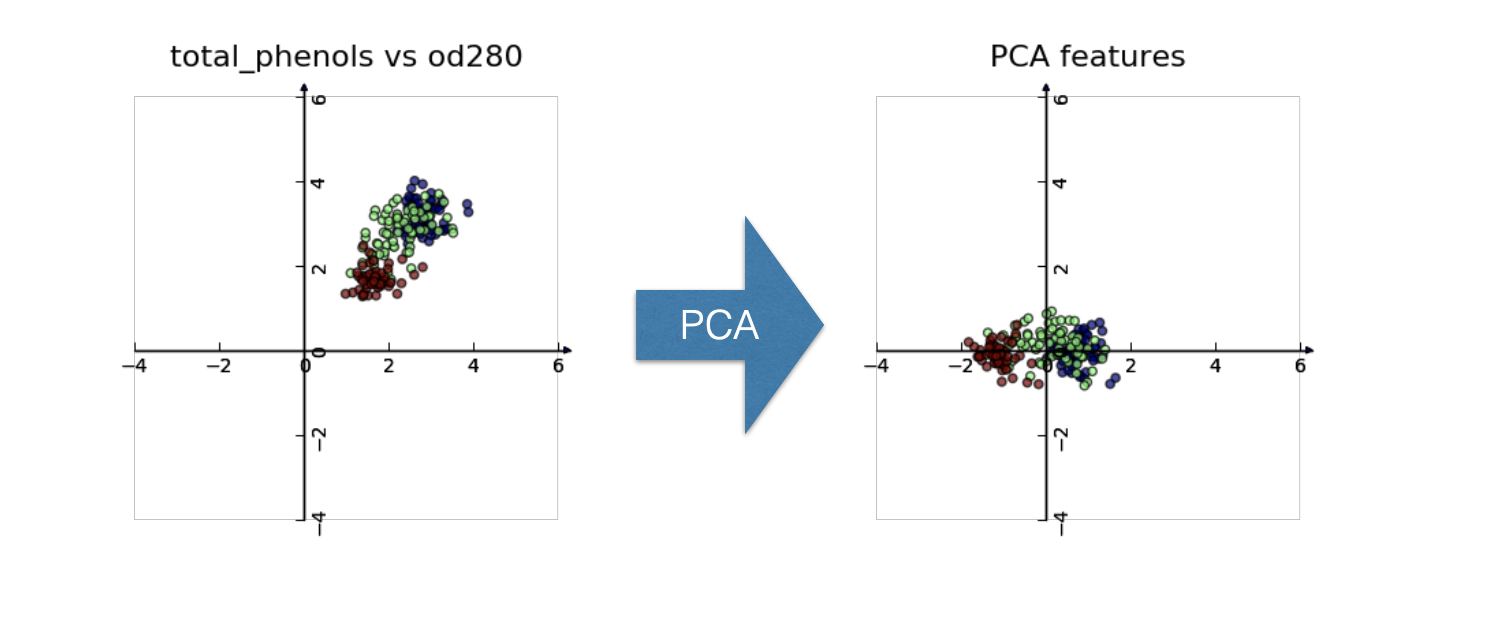
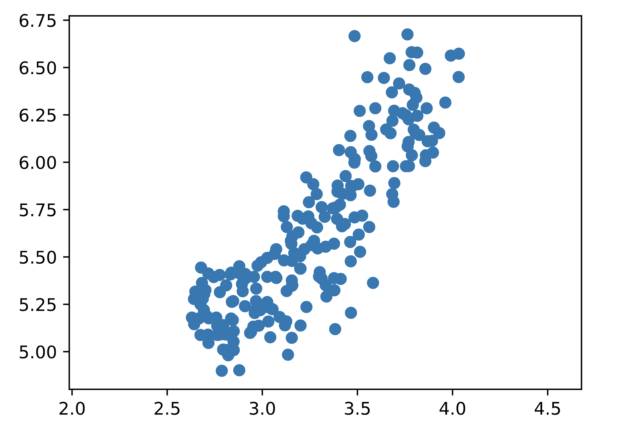
以我们的谷物的长、宽数据为例,
1 | # Perform the necessary imports |
1 | # Import PCA |
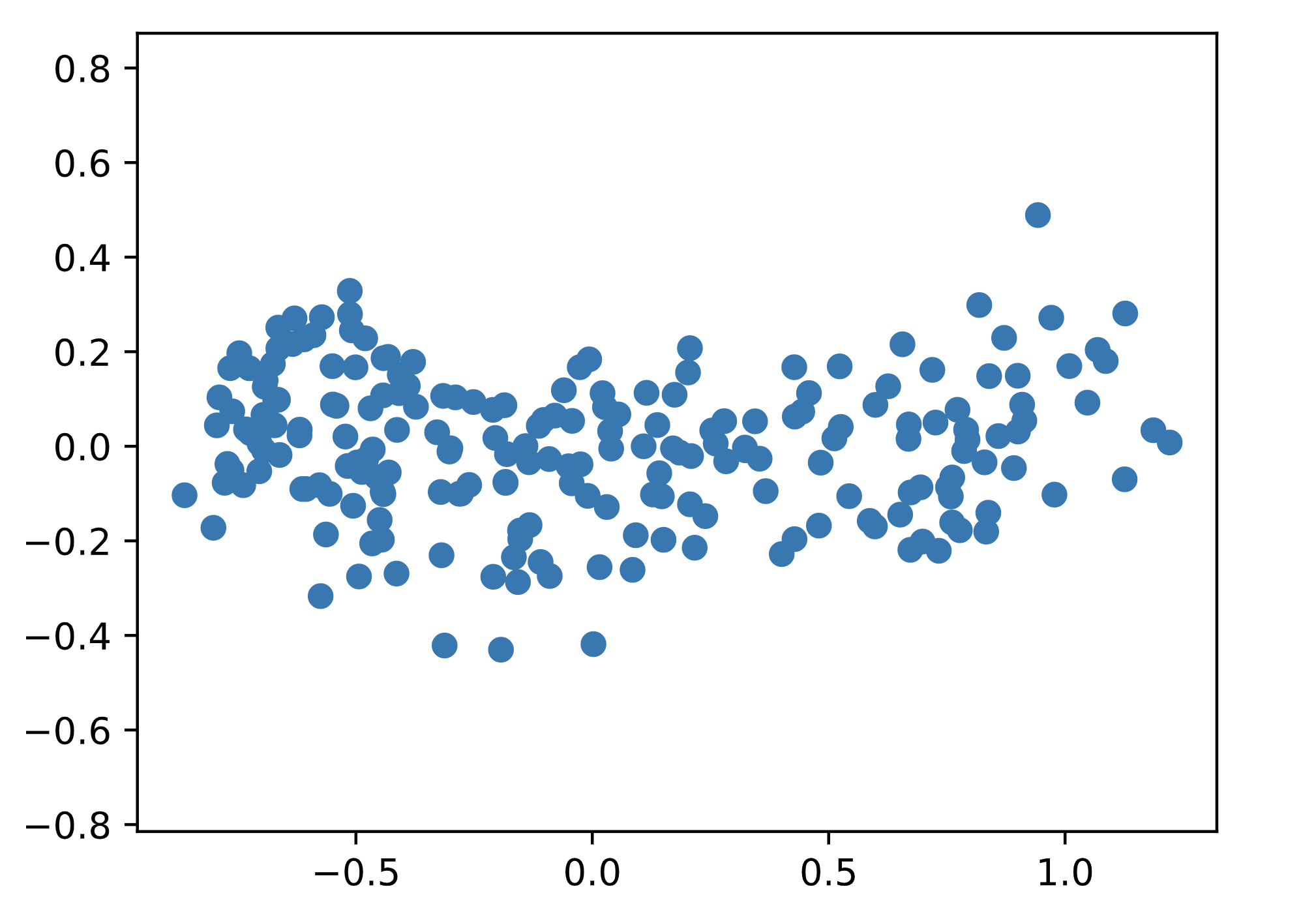
可以看到,谷物的长与宽是有相关性的,即它的叶片越长,宽度也越宽。但在transofor后,数据就与坐标系对齐了。
Intrinsic dimension
Intrinsic dimension 即在降维或者压缩数据过程中,为了让你的数据特征最大程度的保持,你最低限度需要保留哪些features。
它同时也告诉了我们可以把数据压缩到什么样的程度,所以你需要了解哪些 feature 对你的数据集影响是最大的。
比如我们衡量电脑性能,我们可以把键盘鼠标这些feature去掉,但是cpu、gpu、内存性能这些你肯定要保留对不对?cpu、gpu、内存性能,这就是我们说的 features required to approximate it。
但有的人说,我觉得硬盘也得加上去,这样我们的 intrinsic dimension 就从 3 增加到4了。
所以你看,intrinsic dimension 数量是一个视不同情况而定的值。
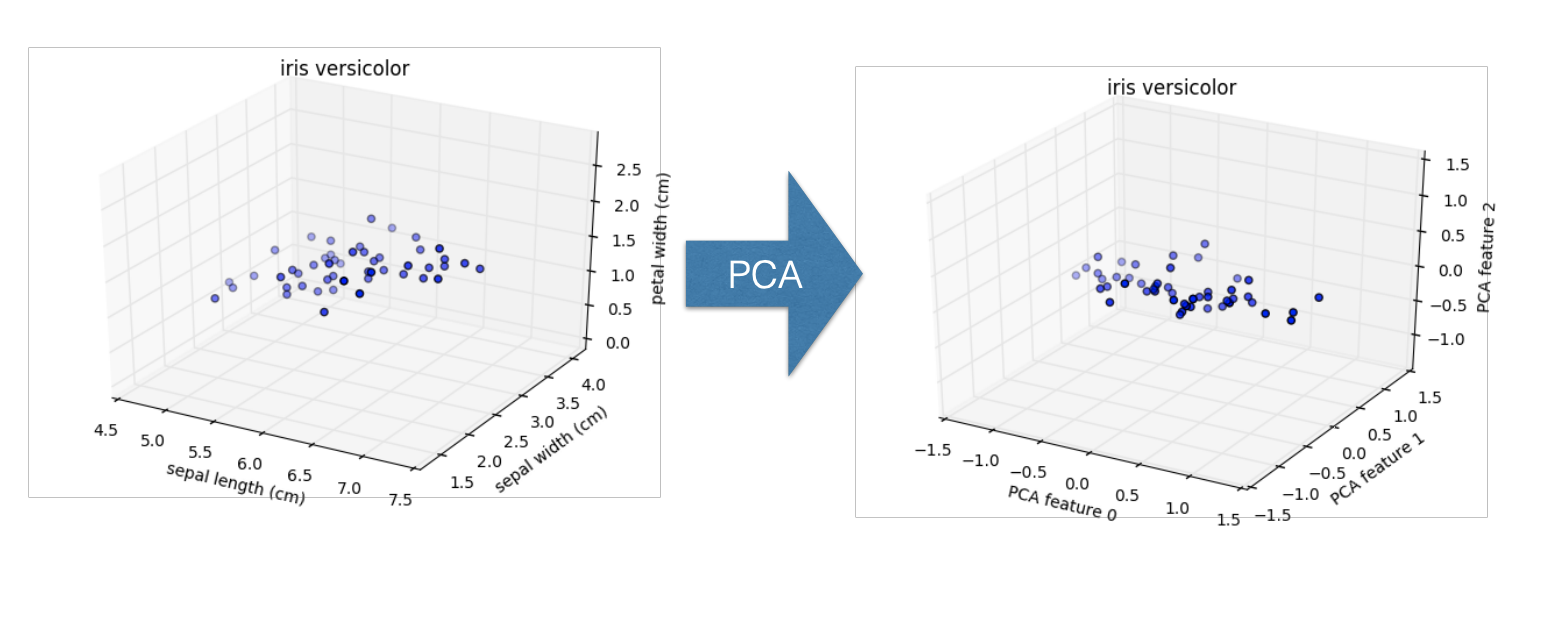
那我们将设为多少比较合适呢?考虑我们的iris数据,我们选择
- sepal width
- sepal length
- petal width
这3个变量,这样我们就可以将它绘制到3维空间,但我们发现它的图像在3维空间是很平的,这意味着某个变量的值的方差很小,也就是说它对整个图像的影响不大,我们只选择另外2个变量,也可以不损失太多的细节。
但scatter图只能表示3维以下的数据,如果我们的 features 有很多个,我们要如何找到那些影响程度大的 features 呢?
这就是 PCA 擅长的地方,我们可以统计 PCA 中那些方差显著的features。
下面是iris数据集各个features的方差排序图:
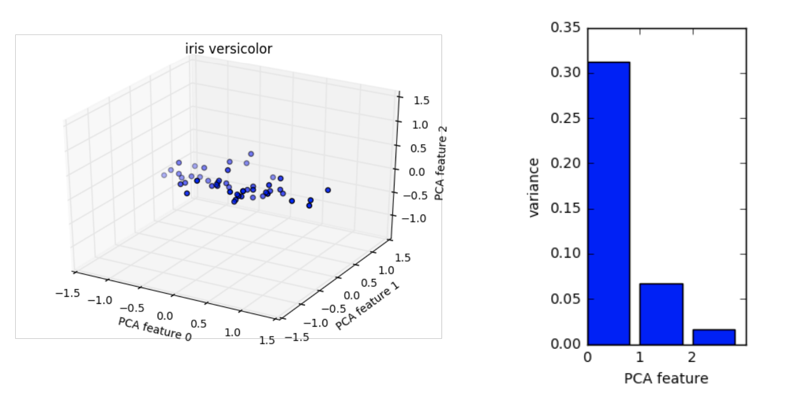
可以看到最后的那个数据方差非常小,所以它对我们数据集的影响完全可以去除掉。
那么如何绘制数据集的 variances 呢?
1 | # Perform the necessary imports |
PCA降维
我们在做数据降维的时候,得指定需要保留的features,即通过指定pca的参数n_components=2, 我们保留多少个features,这可以通过Intrinsic dimension来计算。
我们以iris数据为例,当我们用PCA把数据从四维(petal width,length和sepal length,width)降到2维后,我们再绘制它的scatter图,会发现它们还是分为三部分。
但是对于如字词统计的例子中,我们可能需要用其他的算法来代替,在这种数据中,每一行代表一个文档,每一列代表某个固定词组(fixed vocabulary)中的词语.
我们会统计,每个词语在每个文档中出现的次数array。不过,只有少数的词语会出现很多的文档之中,大部分词语在某些文档中的出现次数都是0,这样的array叫做sparse(稀疏的),sparse array中大部分的值都是0.
我们使用 csr_matrix 来代替 numpy array 去处理这样的数据。
csr_matrix 只会保存那些非0值,这样就更方便,但是PCA不支持 csr_matrix,我们需要用 TruncatedSVD 来代替 PCA。
TruncatedSVD 的效果与 PCA 是一样的,只不过它接受 csr_matrix 数组,除此之外使用方法都是一样的。
示例,我们来对一组词语进行分词操作,我们的词组如下:
1 | # data |
1 | output: [[0.51785612 0. 0. 0.68091856 0.51785612 0. ] |
NMF
NMF与PCA一样,都是降维算法。不过NMF不能用于所有的预测,只能用于非负值。
NMF会将数据集中的每组数据分解并分别计算其和。
考虑字词统计的例子,NMF使用tf-idf来计算字词出现的频率。 tf是词语出现的频率,在每一个document中,如果一个词占整个document中文字的百分之10,那么NMF的输出的tf就是0.1.
而idf用来降低那些常用词的影响,如,的,那个,这个等等。
我们知道,在PCA中,我们定义了多少个n_components,就相当于是保留了多少个features。
在NMF中,它也会去学习数据集的 component dimension。
需注意,NMF的条目,以及features的值,总是正数。
NMF算法使用
1 | # Import NMF |
论文字词统计
Components correspond to topics of documents, and the NMF features reconstruct the documents from the topics
1 | # Import pandas |
用户喜好预测
NMF有一个重要的应用是作为内容推荐,假设我们有一个用户和一部电影,我们想要根据电影的内容做出预测:
| 喜剧片 | 动作片 | |
|---|---|---|
| 小雅 | 喜欢 | 不喜欢 |
| 百货战警 | 3 | 1 |
红番区是动作喜剧片。
现在假设小雅喜欢喜剧片,不喜欢动作片,同时假设我们现在只根据一部电影拥有多少喜剧成分与动作片成分来评价它。
现在因为小雅喜欢喜剧片+3,不喜欢动作片+0,所以它可能给出的评价是 3分 。
我们再来考虑小明的情况:
| 喜剧片 | 动作片 | |
|---|---|---|
| 小明 | 不喜欢 | 喜欢 |
| 红番区 | 3 | 1 |
小明喜欢动作片,不喜欢喜剧片,所以喜剧片的3分不计,动作片1分计入,即小明只给出了1分的评价。
| 喜剧片 | 动作片 | |
|---|---|---|
| 小雅 | 喜欢 | 喜欢 |
| 红番区 | 3 | 1 |
再考虑一个例子:
| 喜剧片 | 动作片 | |
|---|---|---|
| 小刘 | 喜欢 | 喜欢 |
| 让子弹飞 | 1 | 3 |
小刘喜欢喜剧也喜欢动作,所以这部电影他可能会给出1+3,四分的评价。
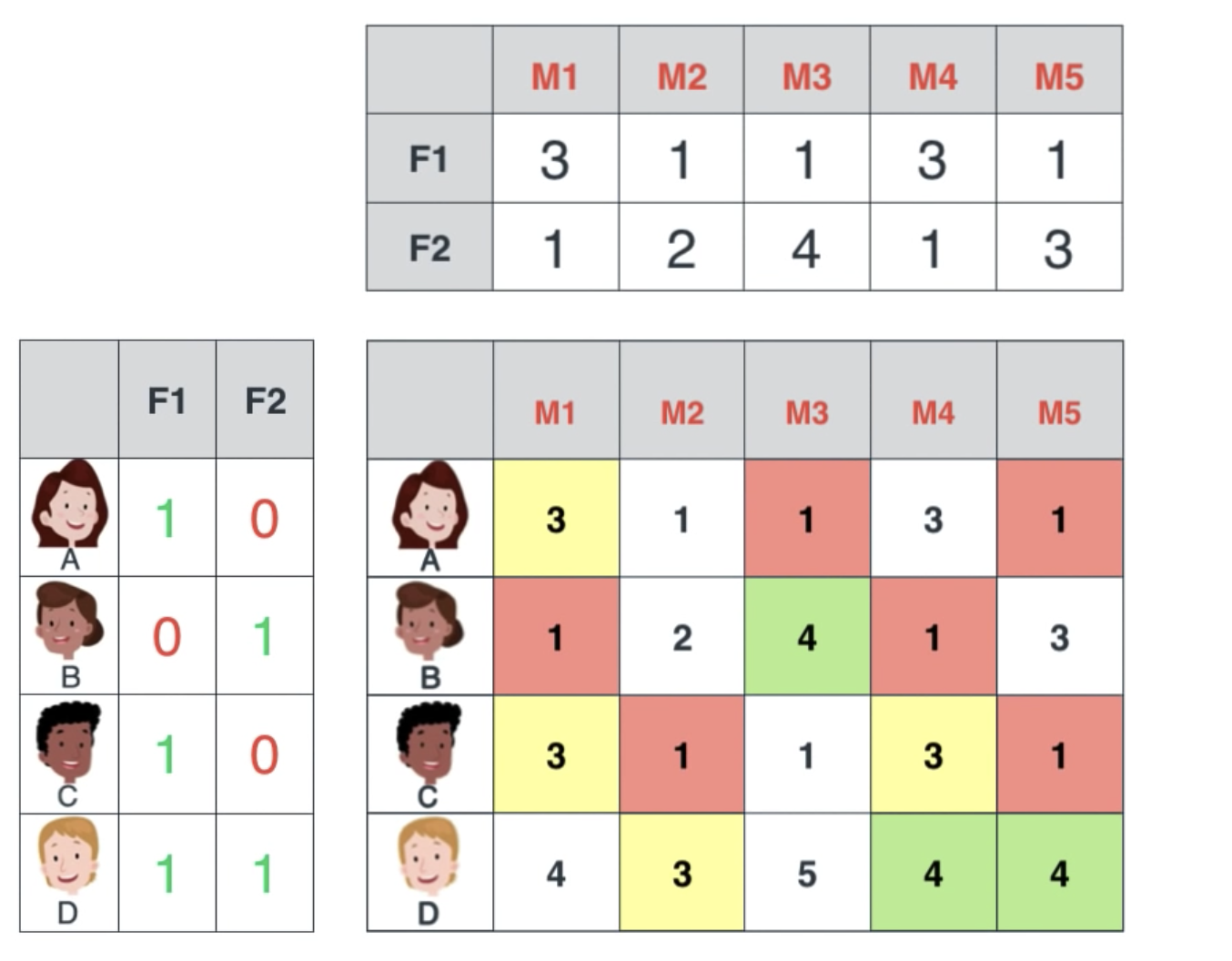
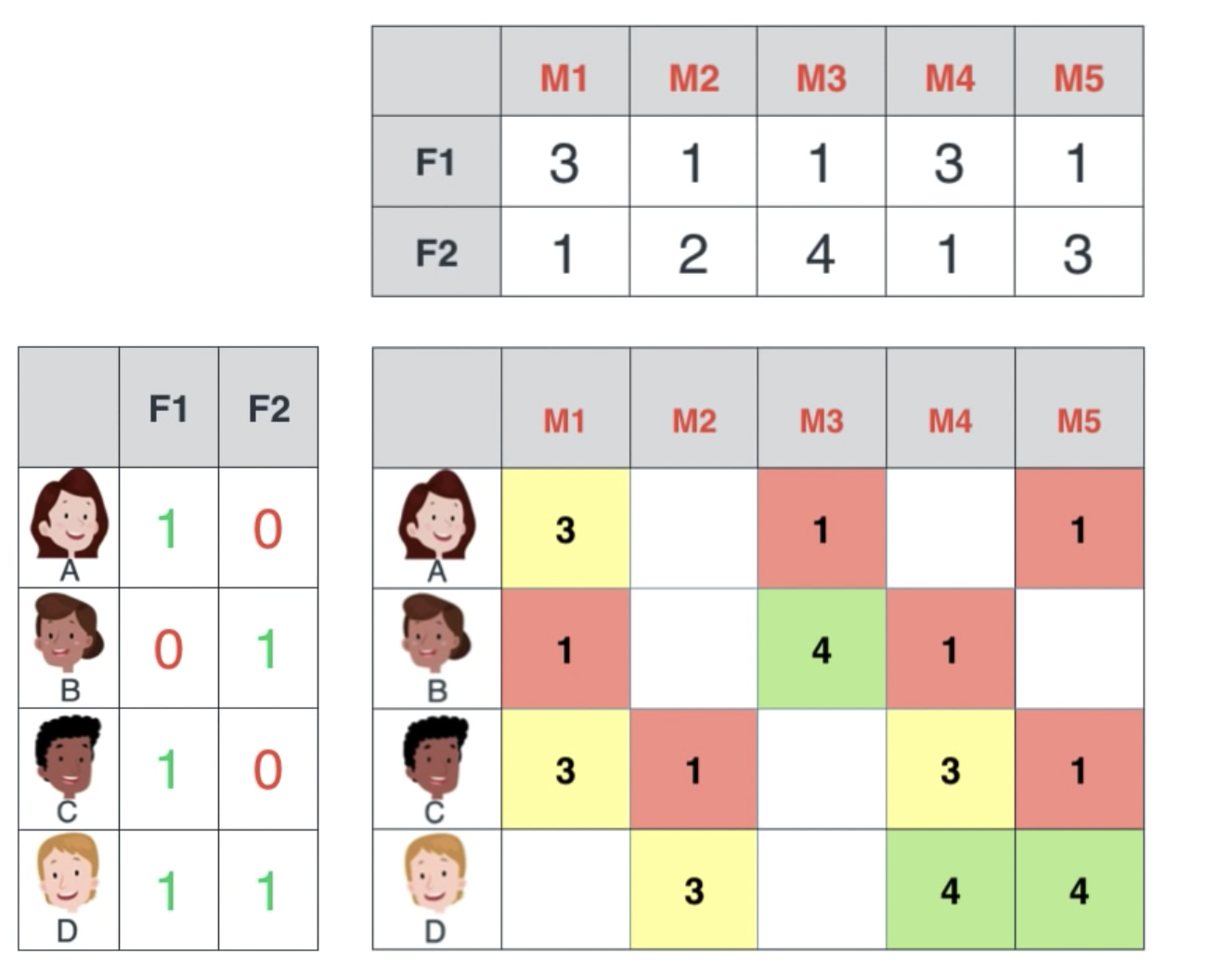
我们把一批电影编号为M1-M5,列表示分别占喜剧与动作的成分,同时把一批用户分类为他们是否喜欢喜剧或动作片。

当我们把左边的两个表结合,就可以得到后面的这个表:
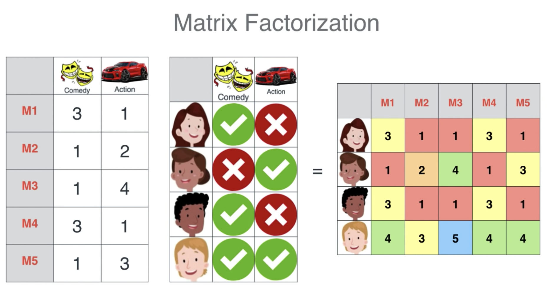
这是通过算点积算出来的,你可以看到:
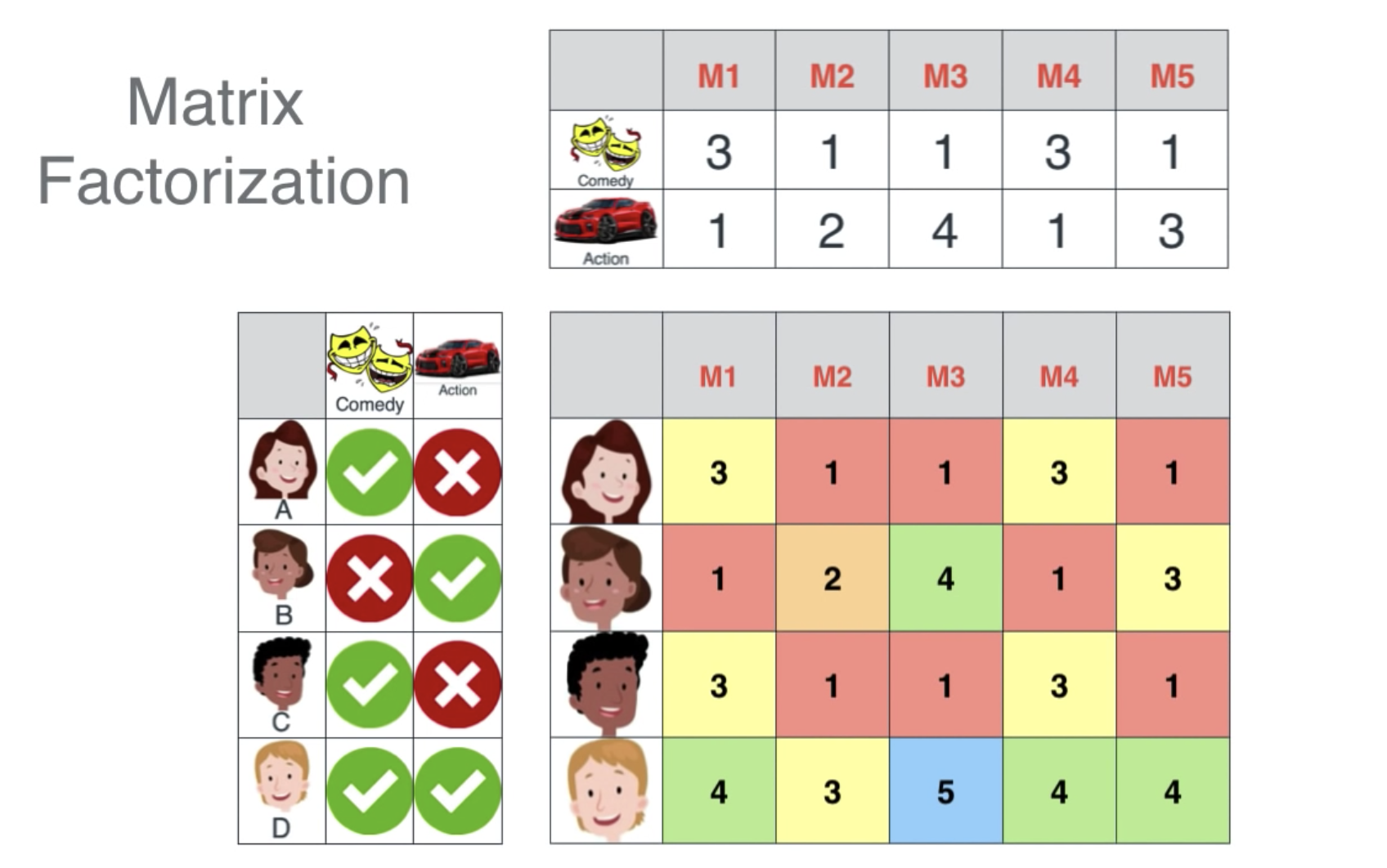
- 有些人的喜好一样,则他们给出的电影评分也是一样的
- 如果两个电影所占的成分差不多,则也会得到一样的评分
- B+C=D,这是因为B的喜欢与C的喜好相反,而D对与这两者都喜欢
- M2与M3的平均值是M5,即M5的喜剧与动作成分是M2与M3的平均值,所以M5的评分也是M2与M3的平均值
上面的这个表叫做Matrix Factorization, 我们要存储这个表是非常费存储的,假设我们有很多的电影与用户,算一下我们需要一个多大的Matrix.

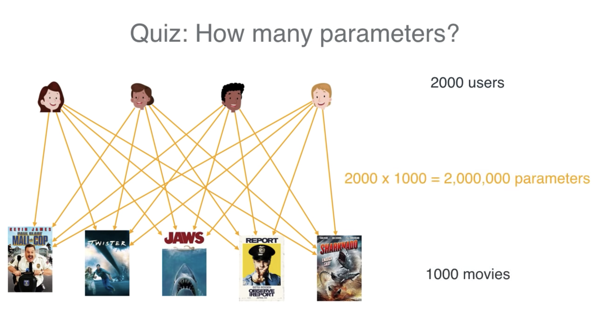
所以我们在存储的时候,只存储用户的喜好与电影的信息,再通过图表演示一下:
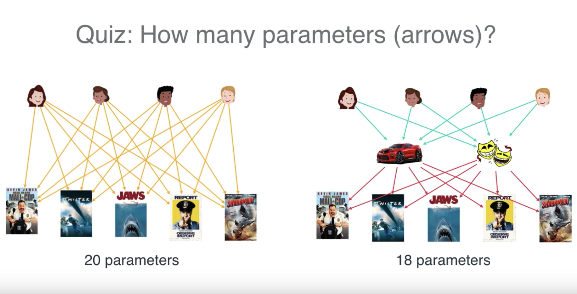
第一种方案是我们直接存储用户对所有电影评分与可能的评分,假设有2000个用户,1000部电影,这意味着200万份数据。
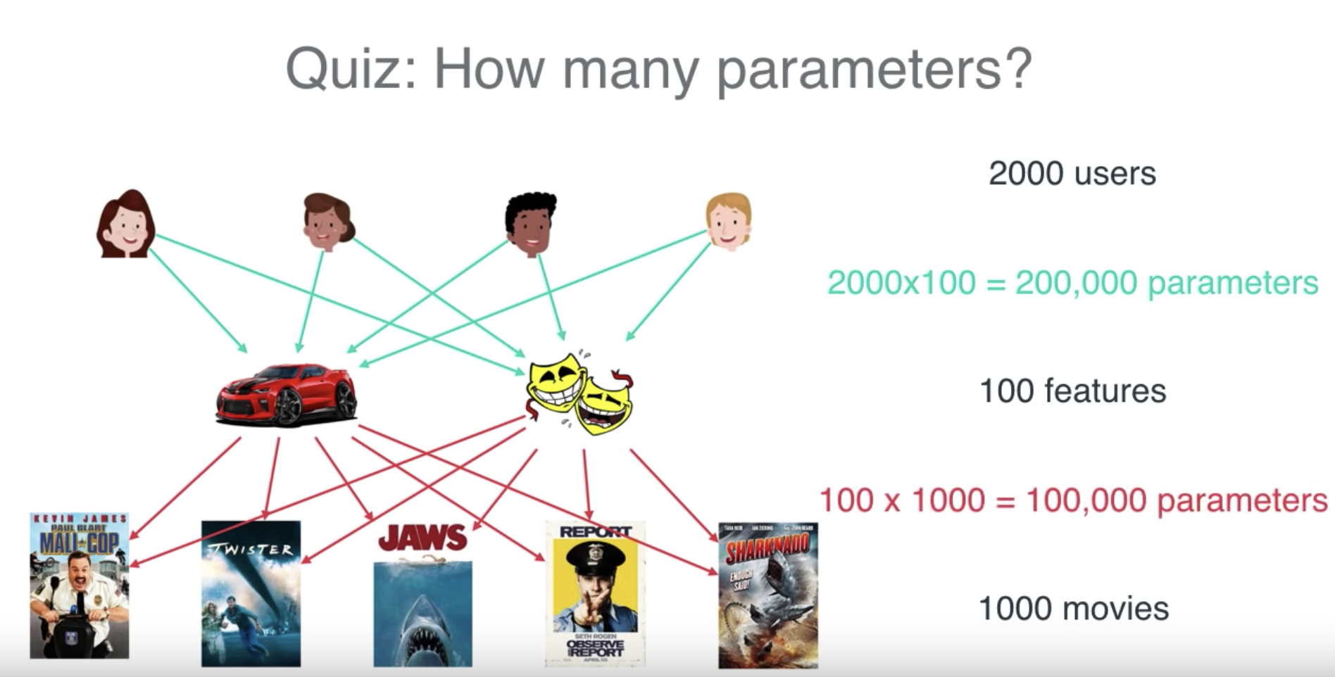
如果我们通过feature计算,则只需要30万份数据
现在我们回到以前,对与NMP算法,其中一个问题是,
如何通过中间的点积,得到两边的数据?就像24可以是2x12,也可以是4x6.
最开始我们可以随机的将两边的数据列出来,算出点积并与手上的点积比对,如果过低,那么我们将相应的用户喜好与电影评分做出调整,直到所有的值接近我们已有的点积中的值。

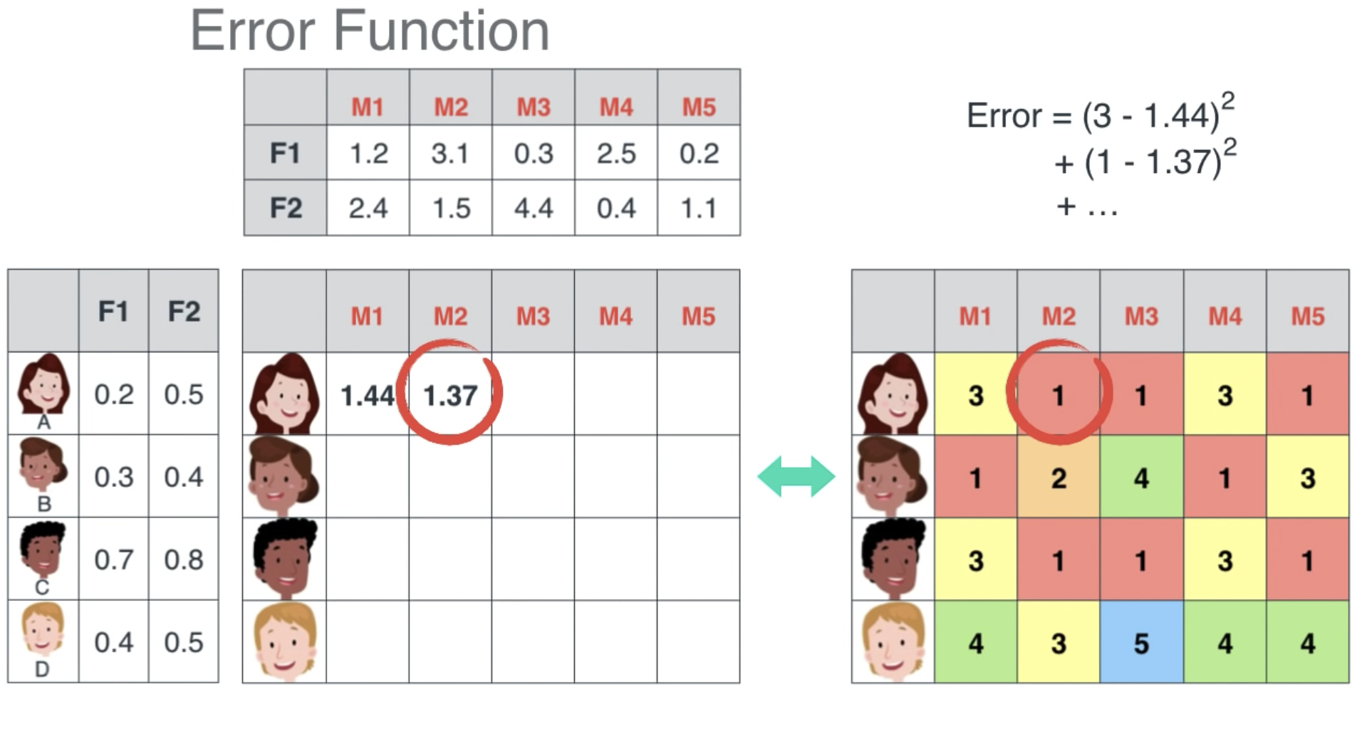
我们算到什么程度,才停止呢?我们需要定义一个error function,它就是告诉机器,你哪里错了,做的还不够,得继续算。
这里的error就是我们手上的数据与机器算出来的数据的差的平方,我们把每个用户或者每个电影的error加起来,error function的作用就是尽量让error的和最小。
在现实的情况中,我们不可能每个用户对每个电影都有评分,所以我们拿到的点积图中间可能有很多空白:
但是我们可以根据这些值算出来用户与电影的属性,进而给用户推荐电影: